The Double Transversality

Every collision table so far has been read in one base at a time. Read two at once and the weights can seem to swallow each other. At seventeen the binary weight is $+1/2$ and the ternary weight is $-2/3$, and their sum, $-1/6$, carries little trace of either. Over a whole table nothing is lost. Tables from bases with no common factor sit at right angles to one another. Their energies add the way the squares on the sides of a right triangle do, and each table can be recovered exactly from the sum. That half of the double transversality is a theorem.

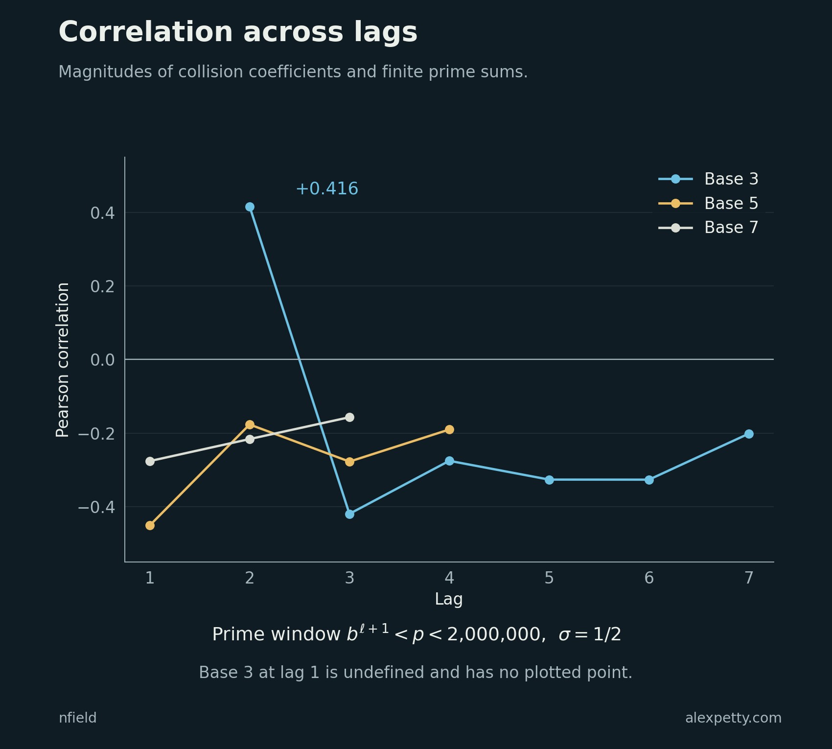
The other half stays inside one base, and it is evidence. The correlation of about $-0.42$ that closed The General Neutrality Theorem came from one base, one lag and one cutoff. It said that big collision coefficients keep company with small prime sums. Following the same pairing to higher lags in bases three, five and seven gives thirteen correlations that can be computed, and twelve of them are negative. The deepest rows grow more negative as the cutoff rises. The one exception, base three at lag two, stays in the record.

The two weights at seventeen come from one count made twice. Write the sixteen fractions with denominator seventeen in base two and again in base three, and compare the first two digits in each row. In binary eight rows open with a repeated digit, and in ternary four do. Subtracting each base’s bin size and family average, the centering of The Centered Collision Sum, leaves $+1/2$ in binary and $-2/3$ in ternary.

Check the two counts at seventeen

The binary matches come from numerators $1,2,3,4$, which begin $0.00$, and $13,14,15,16$, which begin $0.11$. The ternary matches come from $1,8,9,16$, beginning $0.00$, $0.11$, $0.11$, $0.22$ respectively. Only the first two digits of each longer expansion matter here.

For lag one, the baseline is $\lfloor(p-1)/b\rfloor$. At seventeen it is eight in binary and five in ternary. The relevant family means of the reduced table are $-1/2$ and $-1/3$.

$$f_2(17)=8-8-\left(-\frac12\right)=\frac12,$$

$$f_3(17)=4-5-\left(-\frac13\right)=-\frac23.$$

Here $f_2$ and $f_3$ denote the centered lag-one tables. The count uses all sixteen nonzero remainders, whether or not a single reciprocal visits them all.

Two rows, six columns

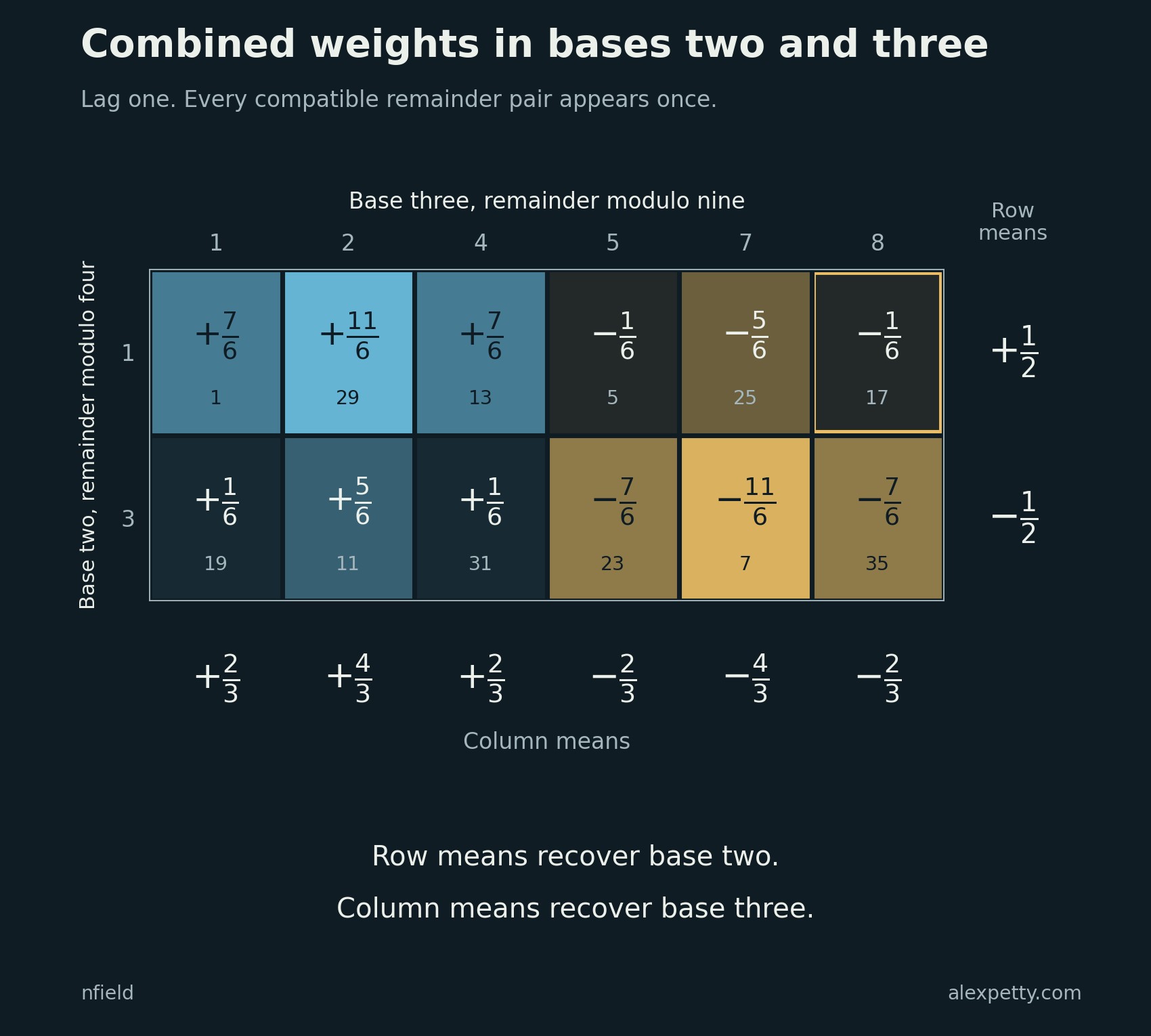
The binary weight of a prime depends only on its remainder modulo four, and the ternary weight only on its remainder modulo nine. It is the same periodicity The Collision Periodic Table found in decimal. Modulo four there are two admissible remainders, one and three, carrying $+1/2$ and $-1/2$. Modulo nine there are six, namely $1,2,4,5,7,8$. Put the two binary choices down the side and the six ternary choices across the top, and fill each cell with the sum of its row’s binary weight and its column’s ternary weight. Seventeen is congruent to $1$ modulo $4$ and to $8$ modulo $9$, so it lands in the upper right corner.

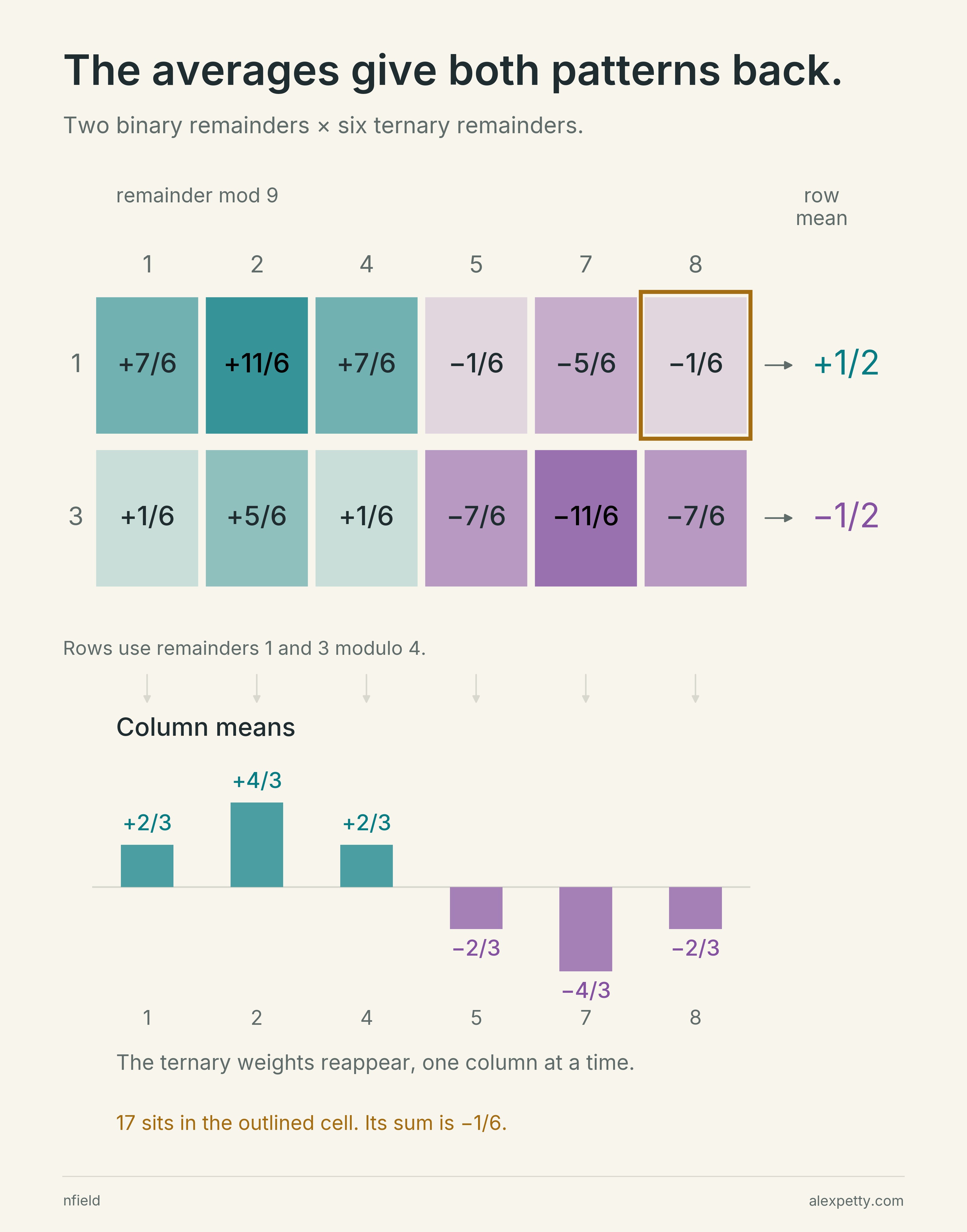
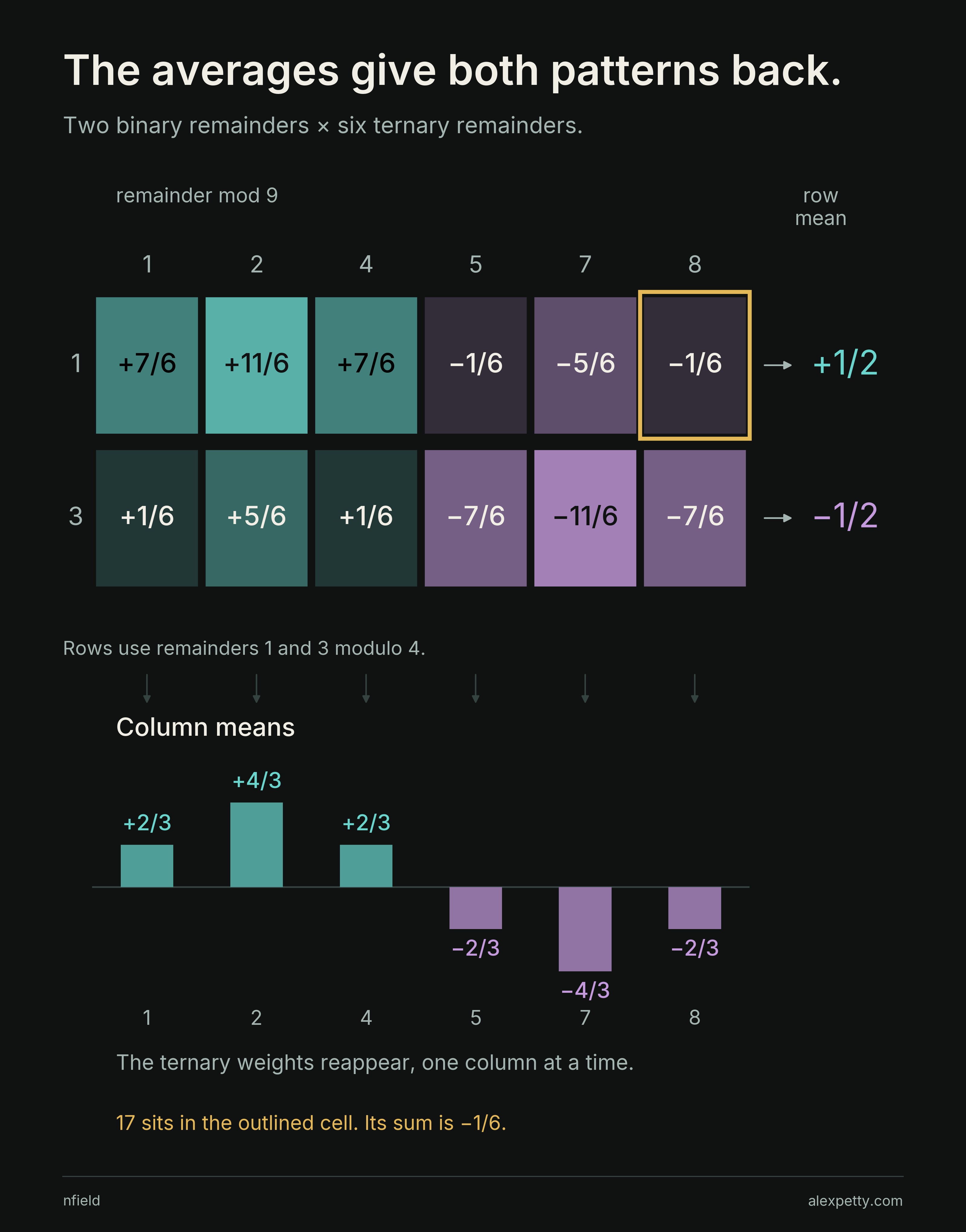
Average across the top row. The binary part is $+1/2$ in every cell while the six ternary weights cancel, so the row averages to $+1/2$. The bottom row averages to $-1/2$, and the binary pattern is back in full. Averaging down a column does the reverse. The binary weights cancel, the ternary weight stays, and all six ternary values come back, the $-2/3$ at seventeen among them.

The rectangle comes from the Chinese remainder theorem. Each pair of admissible remainders occurs exactly once among the twelve unit classes modulo thirty-six. Every cell is a class of numbers, and no distribution of primes enters the recovery. A single sum such as $-1/6$ can’t say which two numbers made it. The twelve sums together keep both patterns.

Read the twelve sums and their residue classes

mod 4 / mod 9	1	2	4	5	7	8	Row mean
1	7/6	11/6	7/6	−1/6	−5/6	−1/6	1/2
3	1/6	5/6	1/6	−7/6	−11/6	−7/6	−1/2
Column mean	2/3	4/3	2/3	−2/3	−4/3	−2/3	0

The row means are $+1/2$ and $-1/2$. The column means are the six ternary weights printed in the last row. The corresponding classes modulo thirty-six are

mod 4 / mod 9	1	2	4	5	7	8
1	1	29	13	5	25	17
3	19	11	31	23	7	35

For example, the two entries $-1/6$ and $-7/6$ in the last column average to $-2/3$. Averaging the six entries in the top row gives $+1/2$.

Three squares

A zero average can hide a large pattern, which is why the squares are worth taking. Square each weight before averaging and the signs stop cancelling. Call the result the table’s energy. The binary table has energy $1/4$. In the ternary table four entries have size $2/3$ and two have size $4/3$, so its energy is

$$\frac{4(2/3)^2+2(4/3)^2}{6}=\frac89,$$

and the twelve-cell sum has energy

$$\frac14+\frac89=\frac{41}{36}.$$

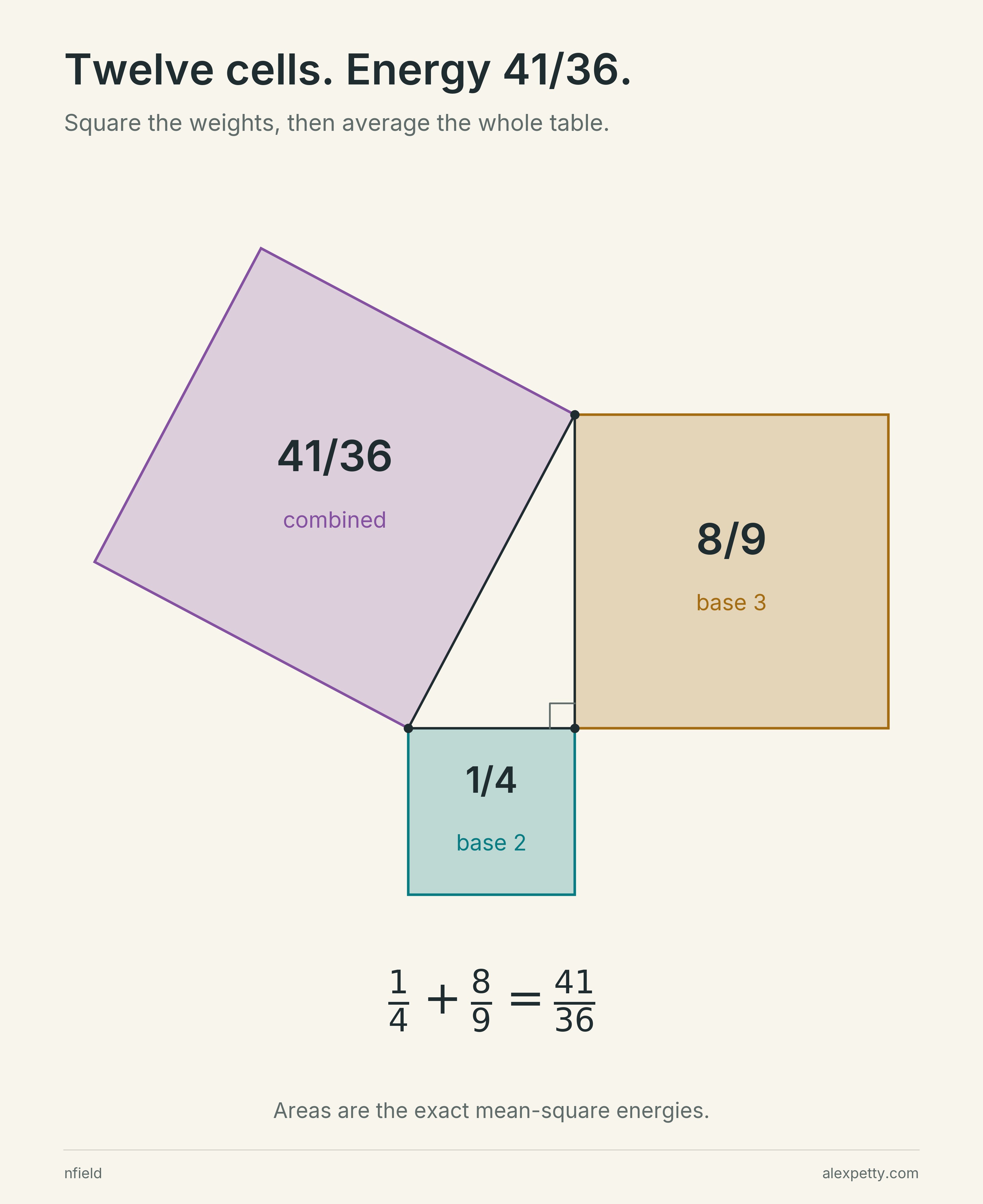
Squaring a cell gives the two squared weights plus a cross term. Averaged over the rectangle, the cross term factors into the product of the two separate means, and both means are zero. That is orthogonality, the algebra behind the Pythagorean theorem, applied to lists of collision weights in place of arrows. At seventeen the two weights nearly cancel. Over the whole table, neither one takes any energy from the other.

The same holds for any finite collection of bases with no common factors, each with its own lag, the distance between the two digit positions being compared. Give the tables complex weights if you like. The combined energy is the sum of the component energies, each multiplied by the squared size of its weight, and averaging over all the other coordinates recovers each weighted component exactly. The proof reads the same at every size, and no prime appears anywhere in it.

Open the joint tables, from twelve cells to 746,496

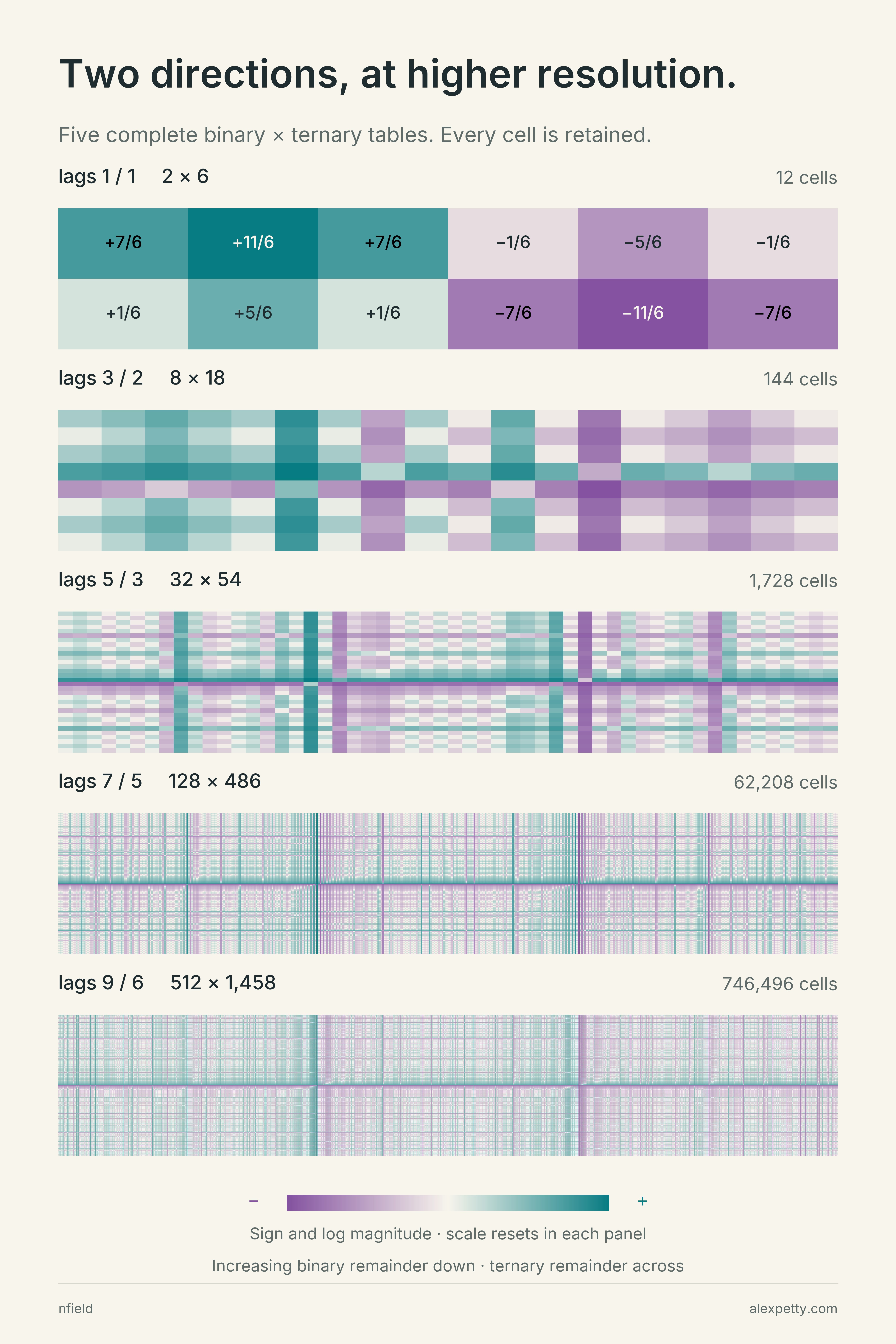
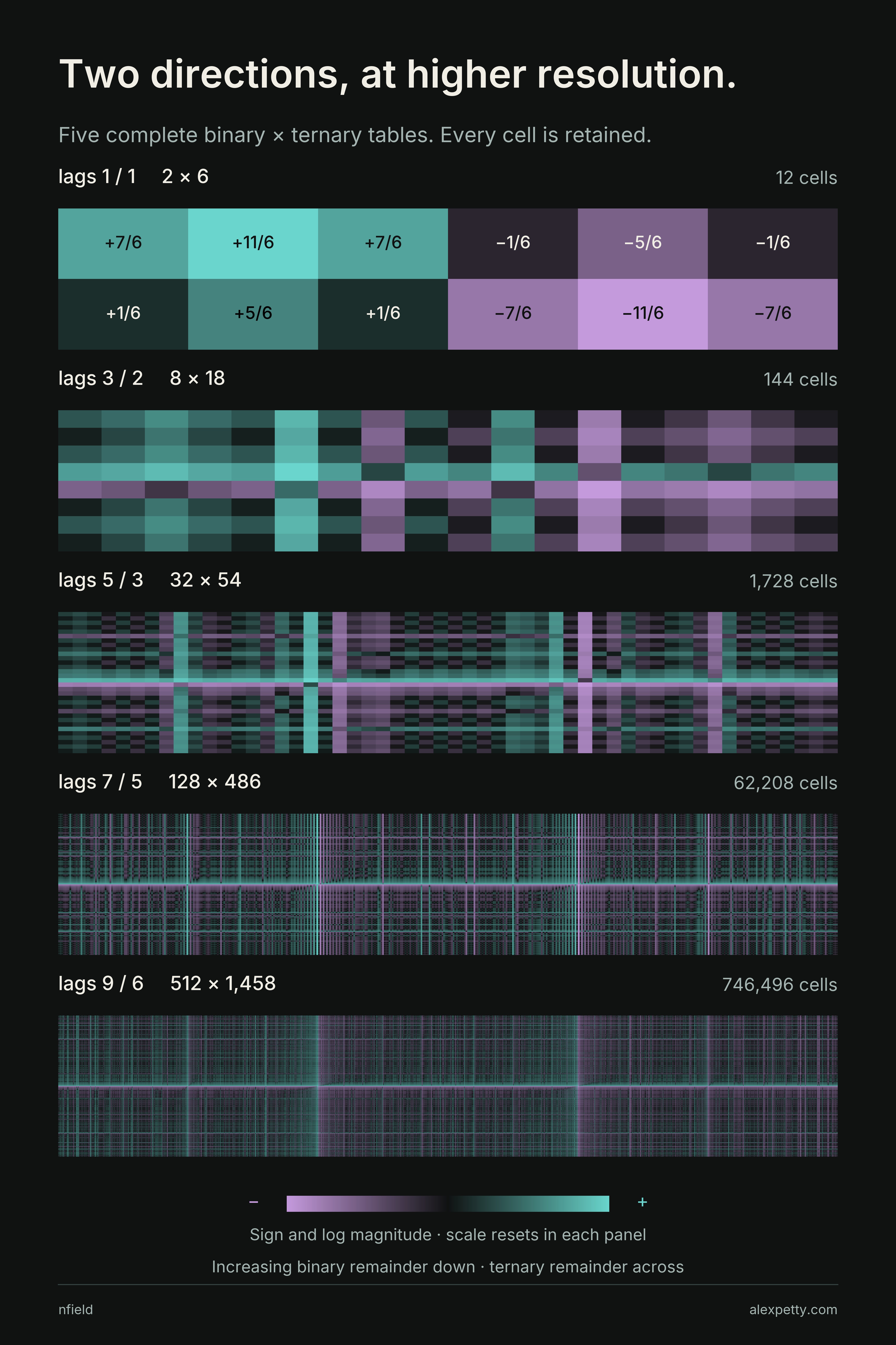
Each panel adds a binary table down the rows to a ternary table across the columns. The lag pairs are $(1,1)$, $(3,2)$, $(5,3)$, $(7,5)$ and $(9,6)$. Row and column means recover the two component tables in every panel. The panels grow, and no primes are involved at any size.

The cross term when bases share a factor

Let the two table moduli be $m$ and $n$. Their common remainder information lives modulo $d=\gcd(m,n)$. Average each table over the entries with the same remainder $u$ modulo $d$, calling those averages $A(u)$ and $B(u)$.

The cross term on the combined modulus $L=\operatorname{lcm}(m,n)$ is exactly

$$\frac1{\varphi(d)}\sum_{u\in U_d}A(u)\overline{B(u)}.$$

The sum runs over the units of the common modulus. For a fixed common remainder, the remaining choices form a complete rectangle. Their average product is $A(u)\overline{B(u)}$. Averaging these products over $U_d$ gives the formula.

Coprime moduli leave only the one-element common quotient, so the separate zero means suffice. Shared factors can retain nonconstant common information and produce a cross term, though they don’t have to. If either conditional average vanishes for every $u$, the cross term is still zero.

Two numbers attached to one character

Inside a single base the pairing works differently. A Dirichlet character assigns consistent signs or complex phases to the residue classes, as in The General Neutrality Theorem. Read the centered collision table with it and you get a coefficient $c_\chi$. Read the primes with the same character and you get a finite sum,

$$P_X(\chi)=\sum_{m<p<X}\frac{\chi(p)}{\sqrt p}, \qquad m=b^{\ell+1},$$

and the collision sum is the sum of their products,

$$F_{b,\ell,X}(1/2)=\sum_{\chi\ \mathrm{active}}c_\chi P_X(\chi).$$

Because the identity is exact at every cutoff, the two ingredients can be compared one character at a time. Plot each active character with its coefficient size across and its prime-sum size up. A point far to the right and near the bottom pairs a large collision coefficient with a small prime sum.

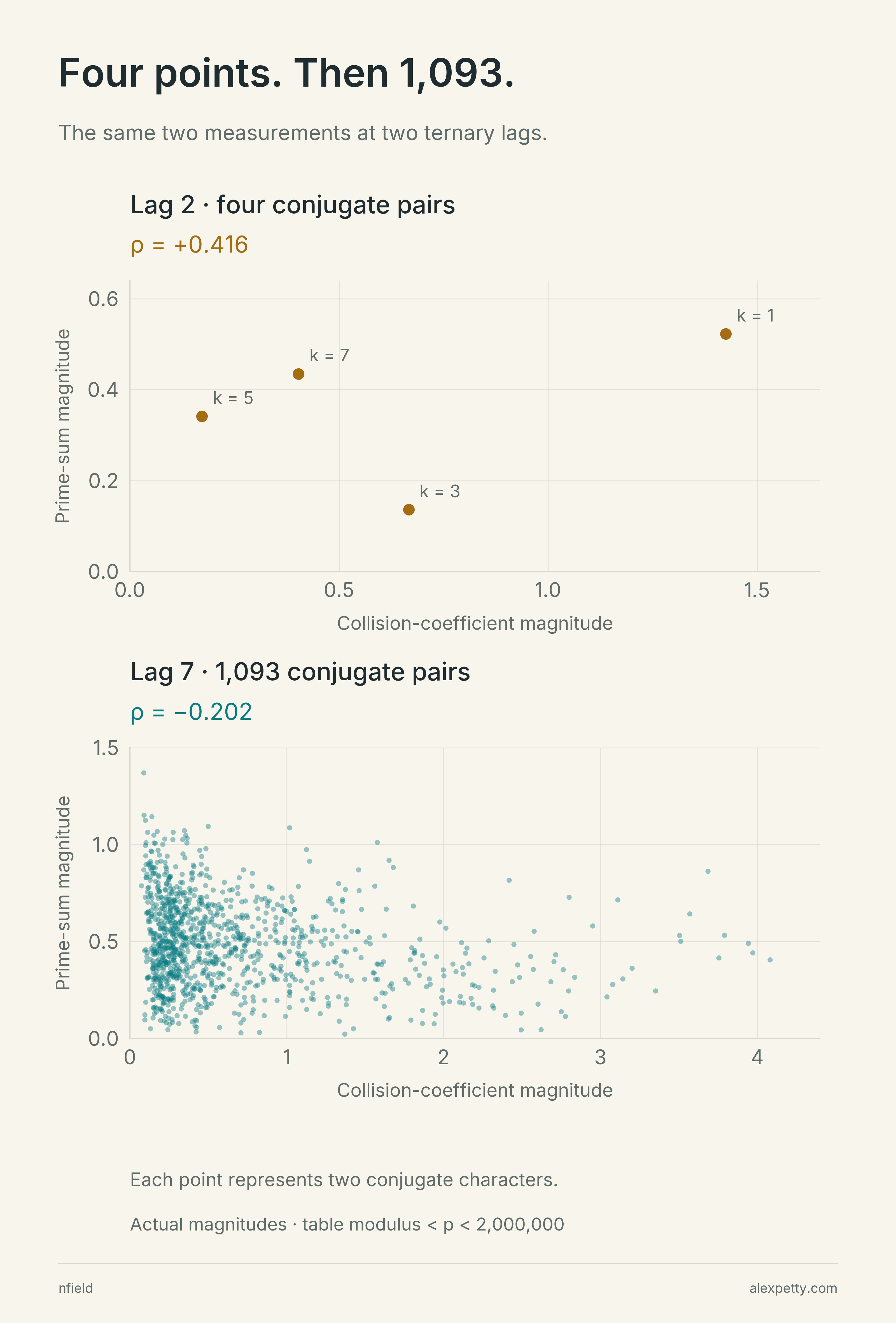
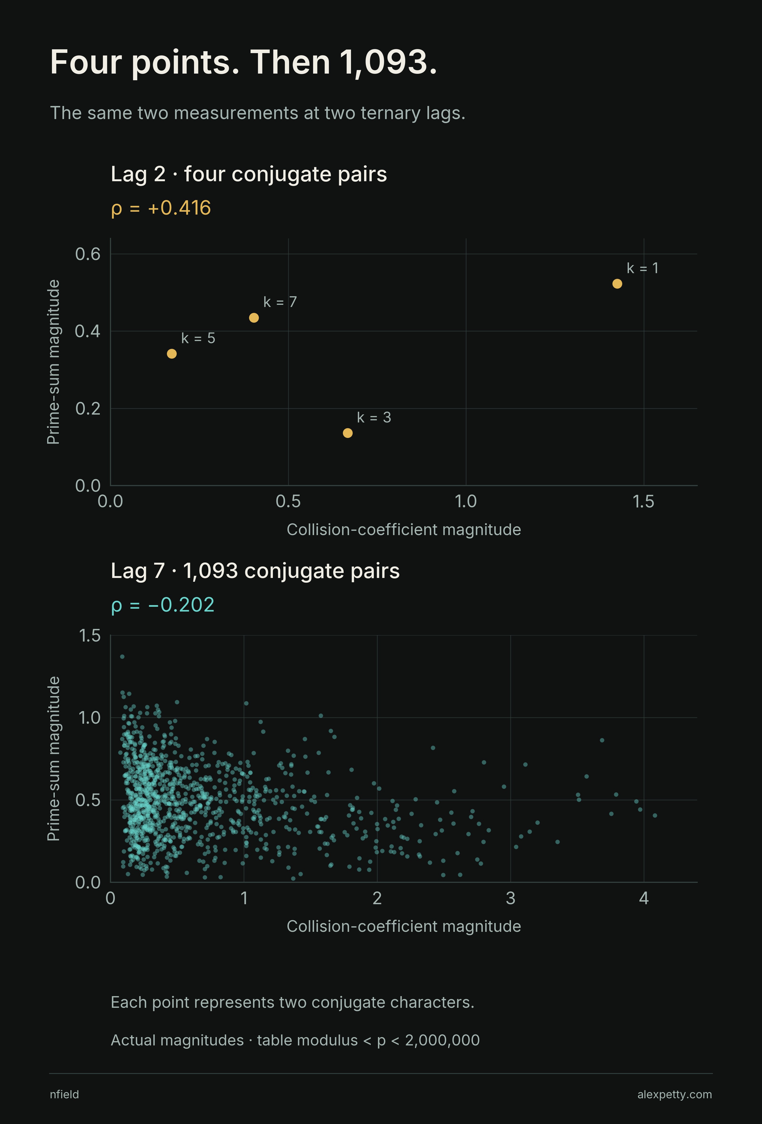
At ternary lag two the four points give a Pearson correlation of about $+0.416$. At lag seven the cloud gives about $-0.202$, so in this window the larger coefficients tend to meet the smaller prime sums, though plenty of points go their own way. Conjugate characters have equal sizes in both coordinates. Each plotted point stands for two terms, and counting both leaves the correlations where they are.

Nothing here splits into separate coordinates the way two coprime bases do. The two numbers belong to the same character, with the table fixing one and the primes the other.

The row that points the other way

Take every prime between the table’s modulus and two million, and run the comparison in base three through lag seven, base five through lag four and base seven through lag three.

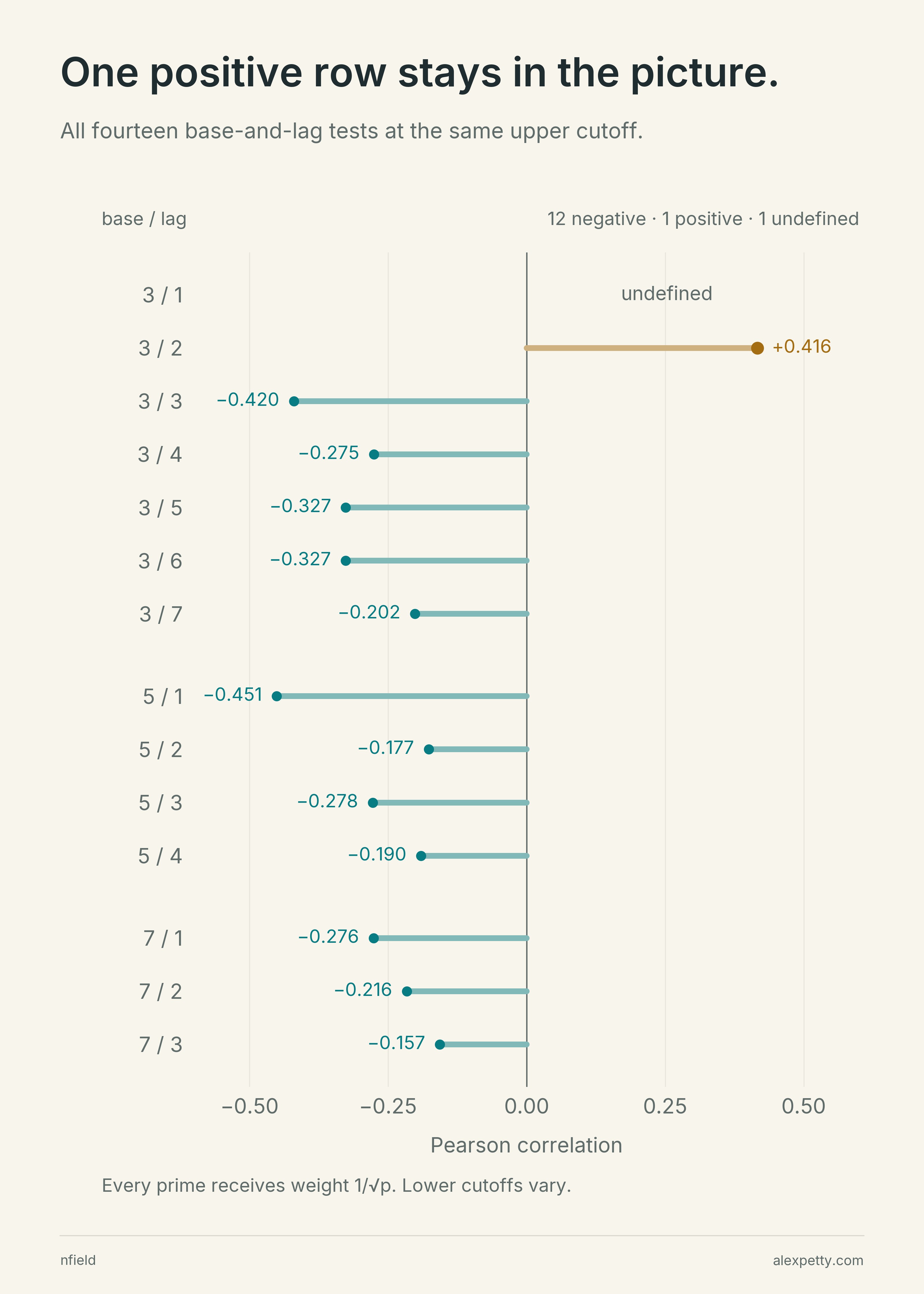
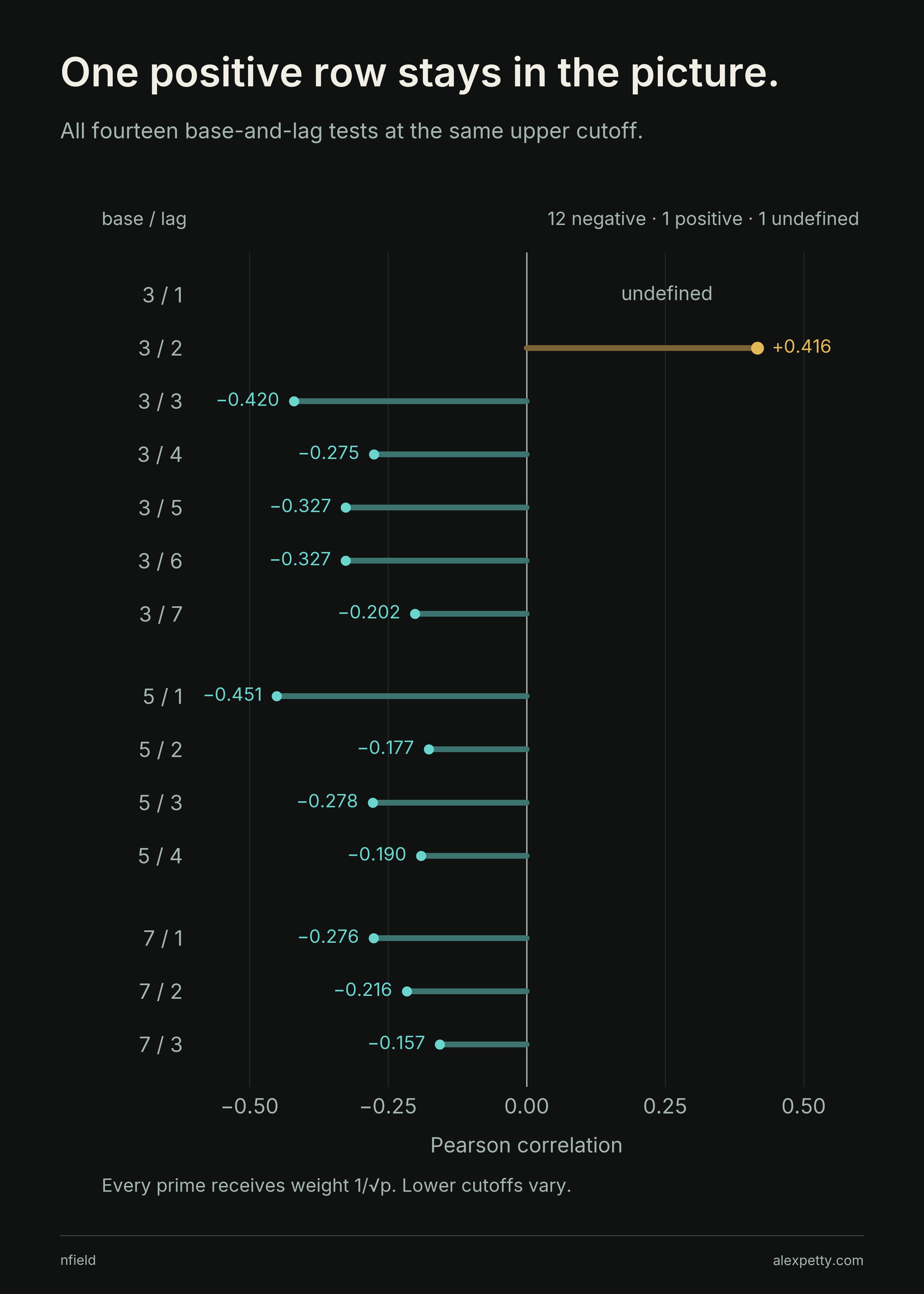
Twelve of the thirteen defined correlations are negative. The exception is the ternary lag-two row from the scatter plot, and it stays in the calculation. Base three at lag one gives no correlation at all. Its two active coefficients both have size $2/3$, so there is no spread across and Pearson’s denominator is zero. Calling that a zero correlation would turn a missing value into a finding.

At ternary lag seven there are $2{,}186$ active characters and one inactive odd one, giving the $1{,}093$ conjugate points in the scatter. The negative association holds as the table grows by a factor of a few hundred. The positive row at lag two is what keeps that from becoming a rule for every lag.

Definitions and all fourteen numerical rows

For units $a$ modulo $m=b^{\ell+1}$, the coefficient is

$$c_\chi=\frac1{\varphi(m)}\sum_{a\in U_m}f_{b,\ell}(a)\overline{\chi(a)}.$$

Fourier inversion expresses $f_{b,\ell}(a)$ as $\sum_\chi c_\chi\chi(a)$. Substitute this into the finite prime sum and interchange the two finite sums. This gives the displayed pairing identity without any convergence assumption.

Even characters and those factoring through the base have zero coefficients. In these fourteen rows, they account for all the inactive odd characters. The numerical retention threshold is $10^{-10}$. The following values use $m<p<2{,}000{,}000$ and exponent $1/2$. Conjugates count separately.

Base / lag	Modulus	Primes	Active / inactive odd	Signed sum	Correlation
3 / 1	9	148,929	2 / 1	+0.618770	undefined
3 / 2	27	148,924	8 / 1	+1.182670	+0.416358
3 / 3	81	148,911	26 / 1	+0.616980	−0.419732
3 / 4	243	148,880	80 / 1	+4.825183	−0.275489
3 / 5	729	148,804	242 / 1	+12.770974	−0.326538
3 / 6	2,187	148,606	728 / 1	+29.145248	−0.326717
3 / 7	6,561	148,086	2,186 / 1	+10.357829	−0.201592
5 / 1	25	148,924	8 / 2	+1.034798	−0.451096
5 / 2	125	148,903	48 / 2	+4.009357	−0.176705
5 / 3	625	148,819	248 / 2	+2.482806	−0.277620
5 / 4	3,125	148,488	1,248 / 2	+15.256874	−0.190394
7 / 1	49	148,918	18 / 3	+1.812203	−0.276190
7 / 2	343	148,865	144 / 3	+7.564420	−0.216332
7 / 3	2,401	148,576	1,026 / 3	+4.583791	−0.156945

The signed sum adds $\operatorname{Re}(c_\chi P_X(\chi))$. The correlation instead compares $|c_\chi|$ with $|P_X(\chi)|$. It discards their phases.

In the ternary scatter plots, $2$ generates the units. The label $k$ means $\chi_k(2)=e^{2\pi i k/\varphi(m)}$. One member of each conjugate pair is plotted. At lag two the four representatives are $k=1,3,5,7$.

Five stopping places

Hold the deepest tested lag fixed in each base and move the cutoff through a quarter million, half a million, one million, two million and five million. All three correlations grow more negative at every step. In base three the value goes from about $-0.052$ to $-0.247$.

The signed sum in that same ternary calculation goes its own way, from $+7.17$ to $-13.77$, then $-1.32$, $+10.36$ and $+4.62$.

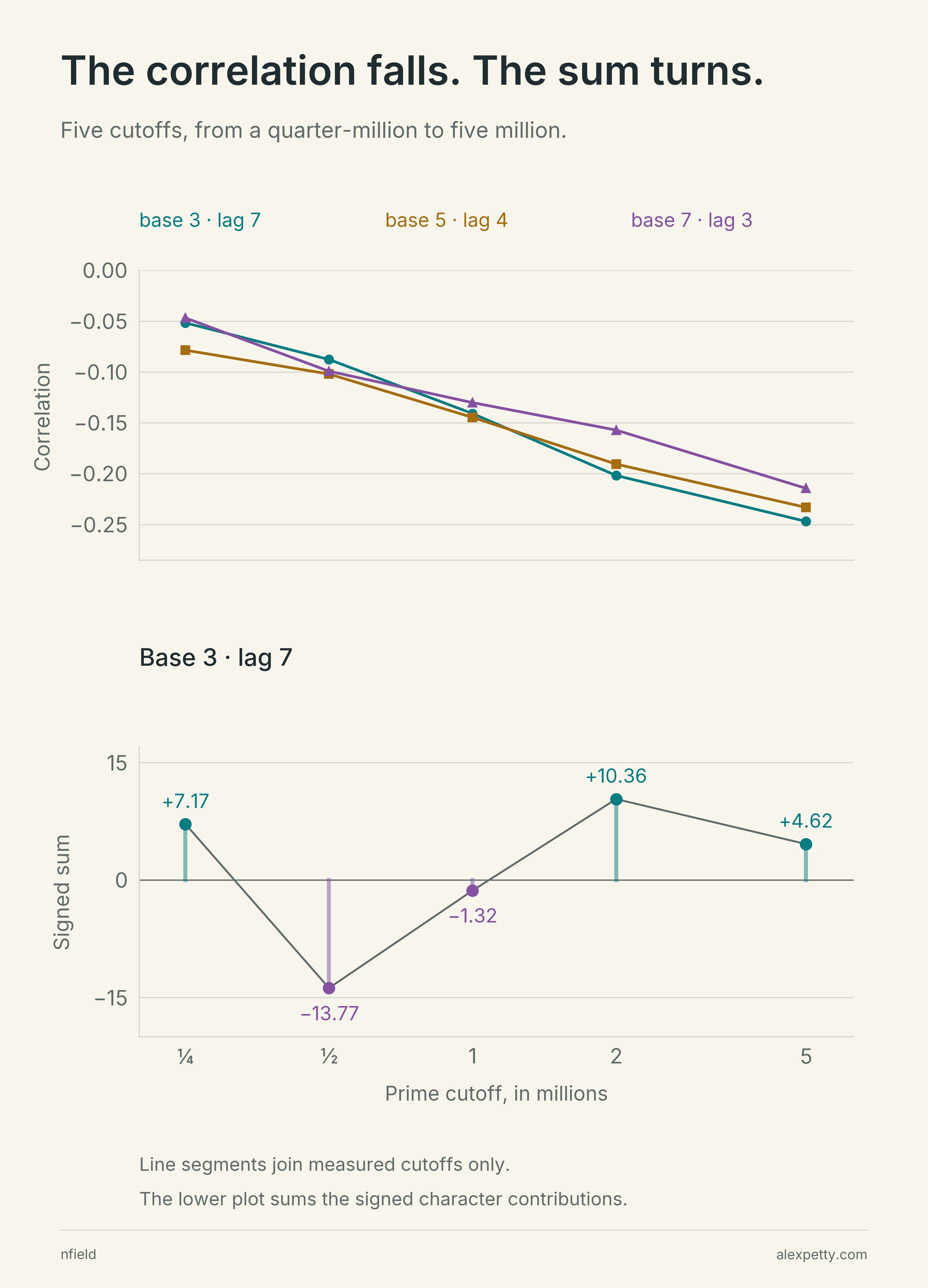
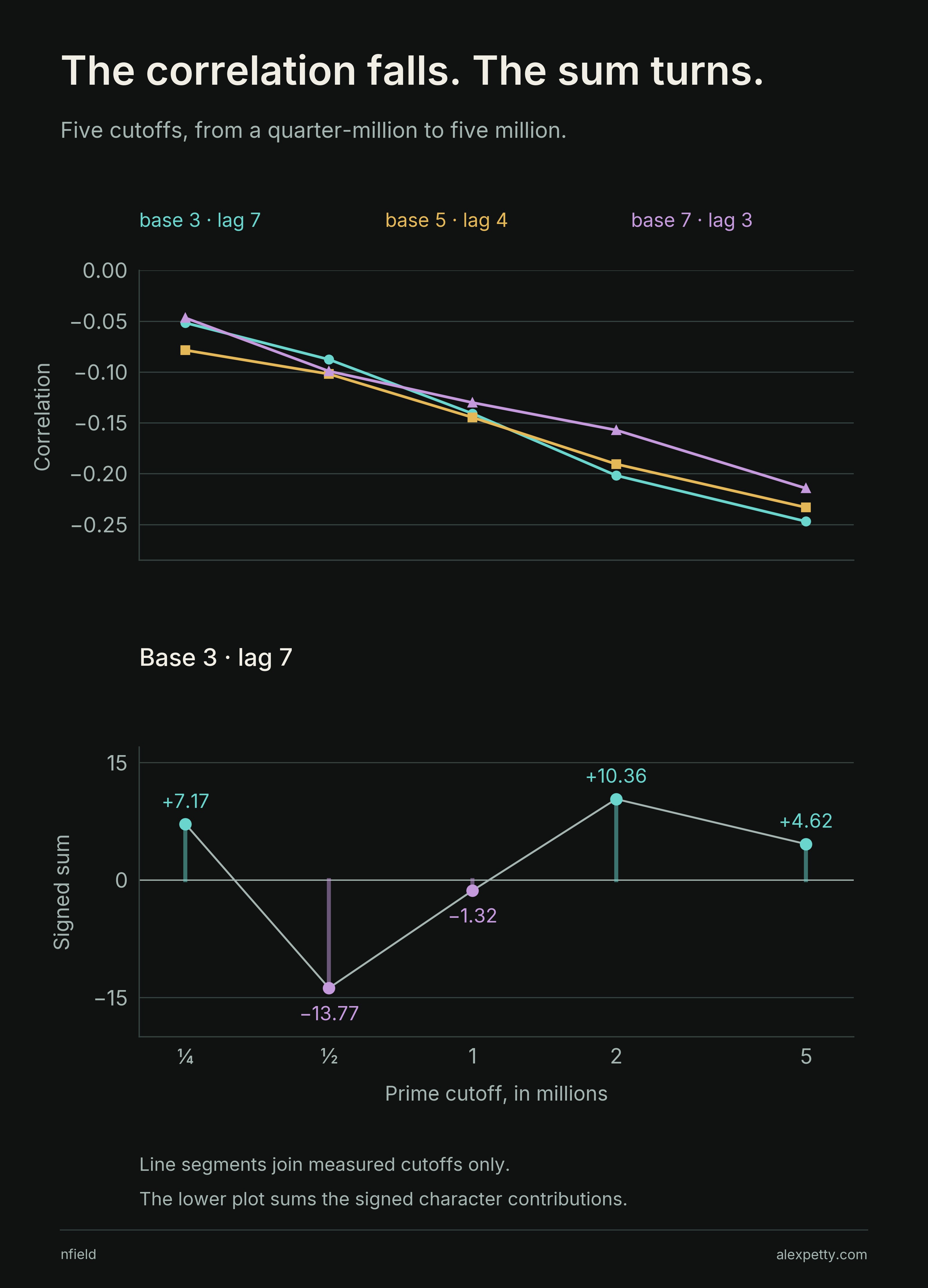
The correlation compares sizes and throws the phases away. The signed sum keeps both, so a steady trend in one doesn’t steady the other. Here the correlation falls at every step while the sum changes sign twice. The direct prime sums and their character decompositions agree in nfield, which checks the arithmetic at these cutoffs and says nothing beyond them. Prime-sum sizes don’t measure distances to zeros of $L$-functions either, and no zero locations enter these plots. The Double Transversality gives the proofs of both directions and the complete numerical ledger.

The rectangle, the lag curves and the cutoff curves, once more

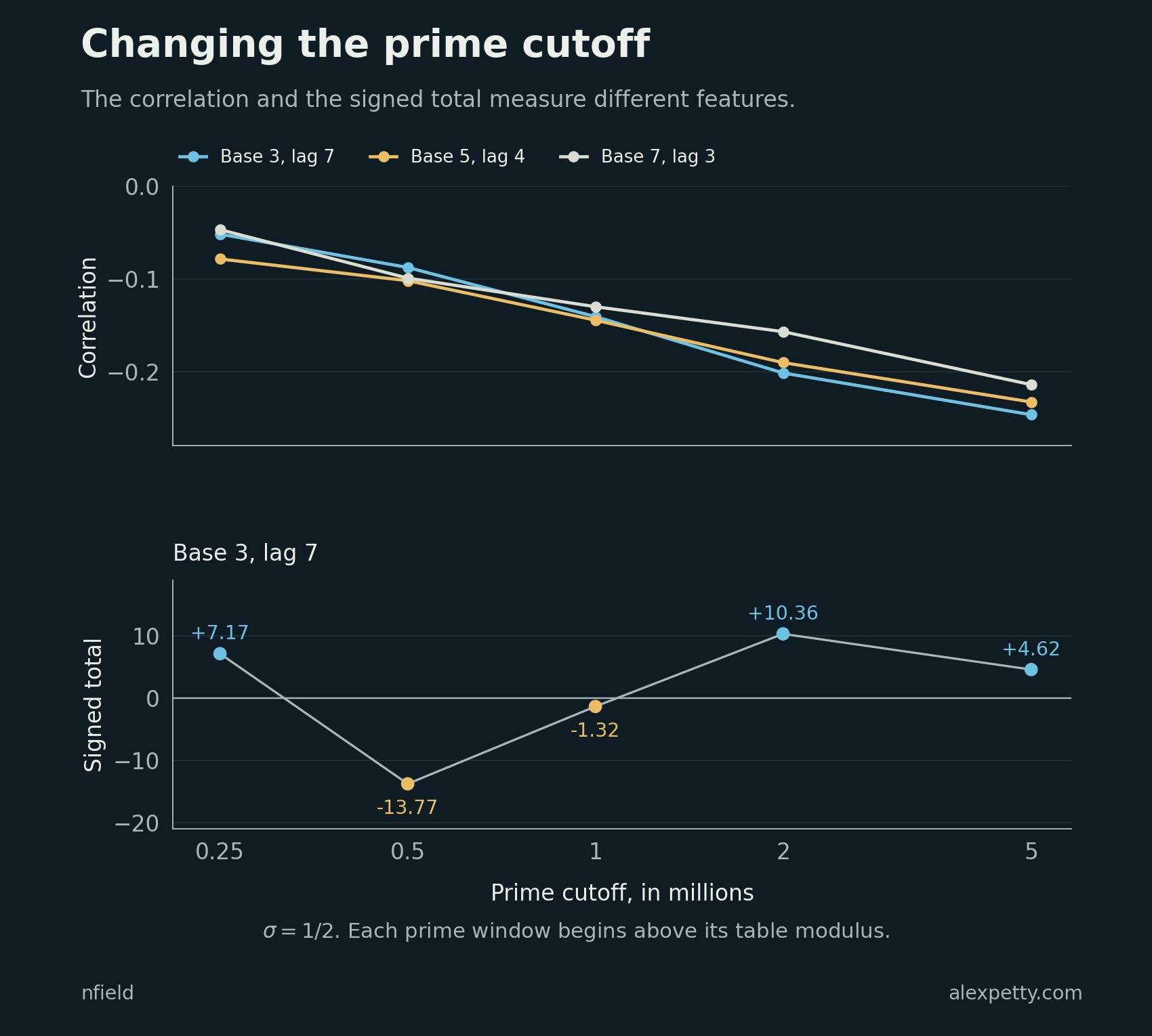
At seventeen the rectangle gives back exactly what went into it, $+1/2$ along the row and $-2/3$ down the column, with no estimate and no primes. Inside base three at lag seven, the correlation reads $-0.052$, $-0.088$, $-0.141$, $-0.202$ and $-0.247$ at the five cutoffs. Whether it keeps falling under a fixed normalization as the cutoff and lag grow is the open half of the pair.